
Developed by Microsoft, Excel may be used to create spreadsheets. For example, Excel can show and produce charts of data input into a spreadsheet, like many other spreadsheet programs It is possible to customize the look of charts by clicking on the Insert section.
Try out a new format or stick with the one that currently connects your data points on a graph. How to connect data points in Excel is explained in this article.
Process of Connecting Data Points in Excel
Begin by entering the information into Microsoft Excel. One column should have all x-axis input, while the corresponding column should hold all y-axis info. A single point’s input should be spread over many cells.
Select all of the cells that contain the newly input data by dragging the cursor over them. After clicking “Insert” in the Charts group, choose the “Line,” then press “Insert” again. Decide on the line chart style that best suits your needs.
Connecting Missing Data Points in Excel
For scatter or line graphs, Microsoft Excel does not link data elements when there are absent data pieces or blank cells. When constructing scatter or line graphs, Excel may handle absent information or missing cells in three distinct ways:
- The value 0 is entered into the blank cell.
- Data points are connected by a line spanning the gaps between them. Without a linking line, each point might display as an individual entry.
- Using the third choice, Excel connects the scatter plot pieces of data, although by default it doesn’t.
As a general rule, using a linking line as an intermediate step is the better alternative. This post will show you how to turn a disconnected line or scatter graph into a connected one by adding data lines where there were previously none.
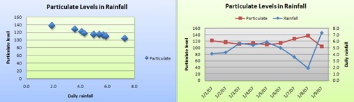
It is shown in the following examples of two batches that are measured sporadically every week. When the data is used to make a scatter graph (or line plot), there are big voids in the information lines. How to link these data points is explained in this tutorial.

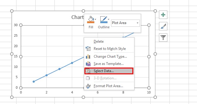
Using your mouse, right-click on a graph or chart. The chart choices appear when you click on it. To pick input, choose the “select data” item from the menu.
When you are in the Select Data Source pane, tap on the “hidden or empty cells” option, which is situated in the lower left edge of the screen.

The “connect data points with a line” item may be accessed by clicking on it. Then hit the OK button to conclude the procedure.

Connected lines will be drawn among data sets. When this option is enabled, any new data or data that is deleted from the chart is immediately adjusted.

Excel does not include an ability to instantly link all data points when creating a scatter or line graph. As a result, any time a line or scatter chart is created in Excel, this quick operation of linking the bent lines between data sets must be completed.
Dot to Line Connection on Excel Scatterplot
There are striking visual similarities between scatter plots and line graphs, particularly when the scatter plots are connected by a connecting line. In contrast, each of these chart styles has a significantly distinct technique of plotting data on the axis of symmetry (also known as the x and y axes).
Using the steps below, you may make a similar-looking line chart. The sample worksheet data was used in the creation of this graphic. You have the option of using the provided data, or your own.
Choose the data you wish to display in a line chart from the drop-down box. Add a Line or Area Chart from the Insert section.

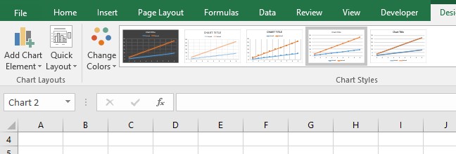
Line with Markers should be selected. The Design and Format tabs will be shown when you click the chart’s region. To utilize a certain chart style, navigate to the Design section and then select it.

Type your desired content by clicking the chart’s title and then clicking the text entry field. If you wish to modify the text size of the graph headline, right-click the headline and choose Font, after which input the size in the Size field. To finish, click the OK option.
The chart’s chart area may be accessed by clicking on it. You may add the legend by selecting it from a drop-down choice of chart components in the Design section, or by clicking on the legend and selecting a position from a range of chart components.
A supplementary vertical axis may be plotted by clicking the set of data or selecting it from a selection of chart components on the Format section, in the Current Selection category, and clicking Chart Elements.
Choose Format Selection in the Current Selection category from the Format section. The Format Data Series task window is shown on the toolbar. Afterwards, choose Secondary Axis in the Series Options and then hit Close.
Include a chart element by clicking the Add Chart Element button in the Chart Layouts group on the Design section.
Choose Primary Vertical from the Axis Title drop-down selection to incorporate a label to the vertical axis. In the Format Axis Title field, choose Size & Properties from the menu to customize the vertical axis heading that you desire.
After selecting Secondary Vertical from the Axis Title drop-down menu, tap on it. Size and Properties may be configured in the Format Axis Title box by clicking Size & Properties.
Each title may be customized by typing in the desired wording and pressing Enter. Pick the chart plot region by clicking on it or by choosing it from a menu of chart components.
Conclusion
Anything you require is at your fingertips with Excel. Excel clients don’t need any extra plugins to make use of graphics. Instead of importing information into another program, you may construct a chart or graph directly in Excel. This tutorial on how to connect data points in Excel should help you generate better visualizations of your data.