You can flip or reverse a pivot table in Excel if you’ve ever desired to. The data supplied by companies is not well-structured or fully prepared for the creation of pivot tables, therefore this might be really handy if you are developing your own. A superior data miner will be able to appropriately unpivot their datasets to qualify them for use in pivot tables. This post will show you how to flip a Pivot Table in Excel for your convenience.
Table of Contents
- Process of Flipping Pivot Table in Excel
- Pivot Table Data Transposition
- Converting Pivot Table Rows and Columns
- Conclusion
Process of Flipping Pivot Table in Excel
In order to flip the pivot table, you must first launch the PivotTable & PivotChart Wizard context menu and then generate a fresh pivot table in Microsoft Excel.
To enter the PivotTable & PivotChart Wizard box, tap the Alt+D+P keyboard shortcuts together. Pick Multiple consolidations ranges from the Where is the data that you want to analyze segment, and PivotTable from the What kind of report do you want to create section. You may also include the PivotTable and PivoChart Wizard function to the Quick Access Panel and then tap on it to activate the preview pane.
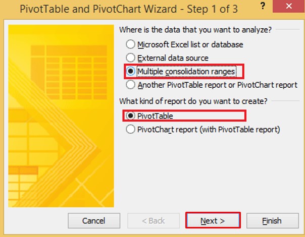
Choose Next to proceed to the next command field, where you may select, I will create the page fields option, and afterward hit Next.

Choose your baseline data, and choose to Add to include the dataset in the list of all available data regions.
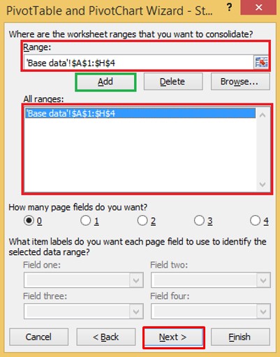
To proceed to the final phase of the Wizard, choose the appropriate preference from the Where do you want to put the PivotTable report segment and press Next. Finally hit on the Finish button.

Assuming that a new pivot table has been established, double-click the final cell in the right edge of the new Pivot table to generate a fresh table in a separate spreadsheet.

Next, on the basis of this new table, construct a fresh pivot table. Choose the entire new table and press the Insert button. Pick PivotTable from the PivotTable drop-down menu.

Subsequently, in the pop-up dialog pane that appears, pick the appropriate choice from the Choose where you want the PivotTable report to be placed portion.
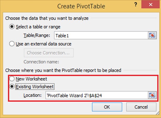
To proceed, select OK. As soon as you’ve completed this, a PivotTable Field List box will appear, and you’ll be able to move the Row and Column fields into their proper sections.
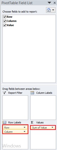
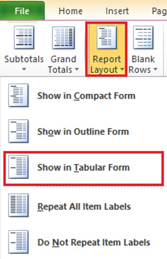
Next, choose any cell in the newly created pivot table and navigate to the Design section, where you will pick Report Layout and afterwards Show in Tabular Form.
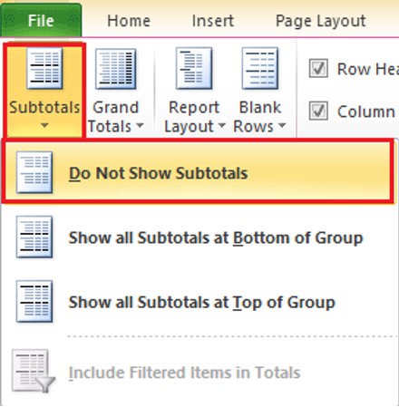
Subtotals will be displayed when you choose Design. Following that, select Do Not Show Subtotals.
The pivot table has now been flipped.

Pivot Table Data Transposition
Here’s the data you’ll be working within this guide: Prices for electronics components are broken down into 4 groups.

Creating a pivot table from this information requires a sampling anywhere inside the dataset. Afterwards, press Insert and choose Pivot table.
Find out whether the range is right and the New Worksheet checkbox is ticked before continuing.
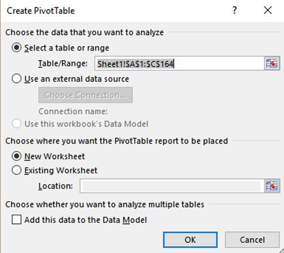
Afterwards, press the OK option. The spreadsheet now includes a pivot table builder. The Category and Part Name must be added as rows, and the Price must be added as values, before the pivot table can be created. The pivot table will be created as a result of this.

Excel displays the pivot table in a small format by convention.
Converting Pivot Table Rows and Columns
Data analysis may be simplified by creating a PivotTable analysis, which simplifies data visualization. Changing rows to columns in a PivotTable is a humble and upfront procedure. Applying this adjustment may make it simpler to examine, based on the sort of data you’re looking into.
- Access the PivotTable report in the Excel worksheet you’d want to adjust.
- Choose “Show Field List” from the context menu by right-clicking on the PivotTable report. PivotTable fields can be viewed here, as well as values, columns, and rows in the PivotTable report filters.
- Choose “Column Labels” from the drop-down menu that emerges when you choose the PivotTable row you desire to convert into a column form. Rows and columns are now shown together.
- Make a column out of whatever field you’d like. You may also alter a row in a PivotTable by selecting “Move to Column Labels.”
- Continue as many times as necessary to keep turning PivotTable rows into columns.
Learn More:
- How To Connect Data Points in Excel
- How To Make a Column Negative in Excel
- How do I Fix the “CTRL+F” Shortcut Not Working in Excel
Conclusion
Flipping data in Excel, i.e., reversing the sequence of the data in a vertical database or horizontal database, may be necessary on occasions. Excel does not have an inherent capability for flipping data, but you may do so in a variety of methods. However, following the instructions in this article on how to flip a Pivot Table in Excel will make it simple for you to do so.

