
There should be no difficulty in converting an integer from a positive to negative. Adding a negative sign to the value is all that’s required. Suppose you have a long list of positive values that you require to turn into negatives.
It would be very time-consuming and, to be blunt, unproductive to apply a negative sign to each individual integer by hand. In order to make all the values negative at once, we’ll need some kind of technique. This post will show you how to make a column negative in Excel to assist you in this endeavor.

Table of Contents
- Approaches for Making Positive Numbers Negative
- Applying Formula
- How to Change Negative Numbers to Positive in Excel
- Applying Excel’s Paste Special Feature
- Conclusion
Approaches for Making Positive Numbers Negative
Assuming we don’t already know how to do it, we can apply a few easy strategies to turn all positive values into negative ones in Excel rapidly.
Applying Formula
If you use the Paste Special approach, you may make positive integers become negative ones by reversing the sign of the integers. To guarantee that only the positive values are transformed to negative, you may use the procedure outlined in this section.
This approach employs a simple formula to turn a column of positive integers to negative. Consider the given set of numbers:
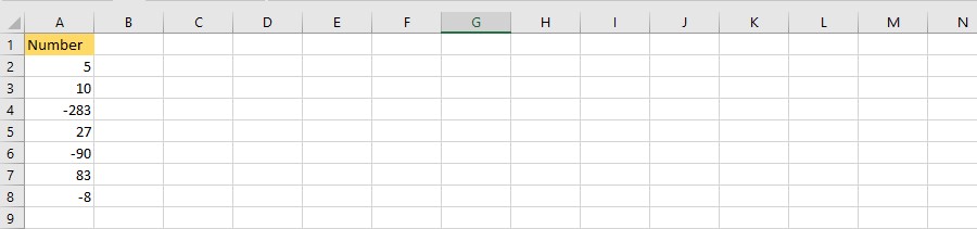
In this list, you’ll find both positive and negative values. Only the positive values should be made negative; the negative values should remain unchanged. To answer this issue, you may use one of two formulas, and both are accurate and beneficial.
Formula 1: Applying the IF Statement
The IF function is used in the first formula. In cell B2, enter the formula and hit the return button:

Once you’ve copied the formula to the fill handle, you may paste it into the remainder of the columns’ cells. Column B should now contain only negative integers.

Column A’s matching value in the formula is verified to ascertain whether it is greater than zero or a positive integer. Adding -1 to a positive value yields the formula’s result; otherwise, it yields a negative one. On the other hand, the formula produces the same result, whether it’s 0 or a negative integer.
Formula 2: Applying the ABS Feature
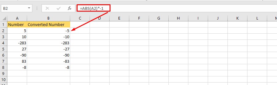
The ABS feature is utilized as the next formula. The absolute value of an integer may be determined using this function. For the purposes of this definition, “absolute value” refers just to the value itself, unaffected by the positive or negative symbol. As a result, enter the succeeding formula in column B2 and hit the return button to transform the values in cell A2:

Once you’ve copied the formula to the fill handle, you may paste it into the remainder of the columns’ cells. As a result, the values in column B should now be entirely negative. It makes no distinction between negative and positive values when using the ABS feature to get the absolute value of an integer. Using the aforementioned method, this amount is then multiplied by -1, enabling you to represent it in a negative format. What you obtain is shown in the following image:
After you have all of your findings, you can duplicate the numbers from column B and paste them over the original numbers in column A using the Paste as Value command. After that, you’re free to remove column B from your spreadsheet.
Read More: How to Change Line Thickness in Excel Graph
How to Change Negative Numbers to Positive in Excel
Applying Excel’s Paste Special Feature
Using this approach, you may alter the signs of all of your integers if they are all positive and you intend them to be negative. Let’s suppose you got these positive numbers:
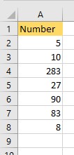
The following are the actions that you must do to turn all of the numbers listed above negative by using the Paste Special function:
- You may write -1 in any empty cell of the spreadsheet. Let’s place it in C2 as an example:

- This integer may be copied by pressing CTRL+C on your keyboard.
- Choose the cells in which you wish to apply the negative sign.

- Using the dialog box, right-click on your choice and choose Paste Special from the drop-down list that emerges.

- This brings up the Paste Special contextual menu, where you may experiment with various paste methods.
- ‘Multiply’ should be selected from the Operation category drop-down field.

- When you hit OK, the signs in all of your chosen cells should be turned negative.
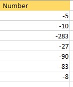
- After that, you may proceed and delete the number -1 from cell C2.
Conclusion
Making each and every input in an excel sheet’s columns may be a tedious and time-consuming task. Being familiar with the various techniques on how to make a column negative in Excel might prove to be constructive knowledge. If you follow the instructions carefully, the techniques listed above should assist you with your operation.