
In an excel worksheet, you can add various numerical information and data to preserve those and calculate. Sometimes, the negative signs before the numbers are unnecessary, but they are somehow added. Eliminating one or two negative signs manually by the “Backspace” or “Delete” button is easy.
But when there are several negative signs, it is valid for you to get devised about how to remove negative sign in Excel. But there are solution methods available to assist you get out of this troubling situation without much hassle.
How to Remove Negative Sign in Excel – 4 Most Effective Methods
In many cases, removing negative signs from the numbers for calculations may become crucial. Even for converting the negative signs to positive, eliminating the negative sign is a must. The process is easy, but things can go wrong if you don’t follow the correct methods.
If you ask how to remove negative values in Excel graph or how to remove negative sign in math, the methods are the same. So now let’s dive into the discussion of the four most effective methods that you can follow in this case:
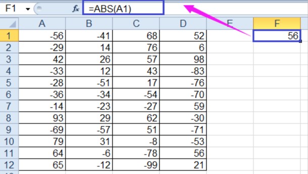
Method-1: Use the ABS Function to Remove Negative Sign
At first, you will have to select a blank cell from the worksheet to start the proceedings. Then, enter the formula of =ABS (Name of the first number cell); for example, you can type =ABS (B2) if B2 is the first number cell.
After typing all these, you will have to hit the “Enter” button to get things going. Then you will see the first number from B2 appearing in the selected blank cell. If the number in the first cell of the worksheet is positive, it will appear as positive in that blank cell.
It will also appear as a positive number with no negative sign if it was negative in the original cell.
Select that newly filled cell and drag the fill handle across the range cells instantly as the number appears. Keep dragging until all the numbers from the parent cells are imported into the new cells. And all the numbers from the new cells you created by handle dragging won’t contain negative signs.
Then you can just copy the new cells and paste them in place of the new cells, and there won’t be any trace of the negative signs.

See also: How Many Chart Types Does Excel Offer
Method-2: IF Function for Checking Removing Negative Signs in Excel
By using the IF function in Excel, you can easily eliminate the negative signs from cells. At first, you will have to select a blank row from your worksheet and locate the first cell and its name. For example, the first number cell is B2, so you will have to type =IF (B2>0, -B2, B2) in that selected blank box.
Then hit the “Enter” button from your keyboard, and you will see the number from the first cell appearing in the box where you typed the IF function. No matter the first the number was positive or negative, it will appear in the new cell as a positive number with no negative sign.
After that, you will just have to drag the file handle to export all the cells from the older cell location. In this case, there will be no negative signs in any of the new cells that you exported a while ago.

Method-3: Use Find and Replace Command to Eliminate Negative Signs
This command is a simple one for eliminating the negative signs from the numbers. The task is quite simple as you will have to select the cells that contain negative signs in front of the numbers. After selecting the cells, you will have to click on the “Home” tab from the top-left corner of the Excel window.
In this tab, you will find a section called “Find and Select” in the upper part of the window. Click on the name, and a small panel with some options will pop up instantly below that section. Next, locate and click on the “Replace” option from that options panel.

As a result, a new small dialogue box of “Find and Replace” will pop up, containing some blank boxes to work with. There will be two sections of this dialogue box, and you will have to click on the second one named “Replace.” After entering this tab, you will see two blank boxes named “Find what” and “Replace with.”
You need to type “-” in the first box to find the cells with this minus sign. At the same time, you will have to keep the following box blank to avoid adding any other signs to the numbers in the cells. After doing all these, you need to click on the “Replace All” option to finally eliminate all the negative signs from the cells you selected.

Method-4: Use Custom Formatting to Eliminate Negative Sign
It is one of the most useful negative signs removing methods as you won’t have to create any new cells. However, you will have to select the cells containing negative signs first and then hit “Ctrl + 1” from the keyboard. It will bring up the “Format Cells” window with various categories.
You need to click on the “Custom” option from the bottom of the category list with various formatting options appearing besides it. From those options, select #,###;#,###, and hit the “OK” button situated down to that “Format Cells” window.
By doing so, all the negative signs from the cells of your Excel worksheet will be removed.

Final Thoughts
While editing your Excel worksheet, you may require to eliminate the negative signs from the numbers. But if you are new to Excel worksheets, it is mandatory for you to learn how to remove negative signs in Excel first. There are several effective and proven methods you can apply to complete this action of negative sign removal.
Some will require adding the new number of cells, or some can eliminate the negative signs from the original cells. All these methods are effective if you can perform them properly by following the instructions.